GLM.Interactions

Reading: Goldburd, M.; Khare, A.; Tevet, D.; and Guller, D., "Generalized Linear Models for Insurance Rating,", CAS Monograph #5, 2nd ed., Chapter 5. Section 6

Synopsis: In this article you'll learn what an interaction is and be able to describe the three types of interactions between variables which can occur. You'll also learn how to read GLM output to determine if an interaction is significant and find the appropriate model relativities.

Study Tips

Alice: "This material is challenging and historically hadn't been tested much. However, the CAS is putting more emphasis on GLMs and modelling so you really need to understand this material. I've broken it down into smaller pieces and filled in most of the details glossed over in the text."

Estimated study time: 16 Hours (not including subsequent review time)

BattleTable

Based on past exams, the main things you need to know (in rough order of importance) are:

Know if the GLM model output contains an interaction.
Be able to calculate variable relativities from GLM output.
Be able to re-base a continuous variable within an interaction.
Know the advantages of re-basing variables.

Questions from the Fall 2019 exam are held out for practice purposes. (They are included in the CAS practice exam.)

reference	part (a)	part (b)	part (c)	part (d)
Currently no exam questions for this reading

Full BattleQuiz

Excel Files

Forum

You must be logged in or this will not work.

In Plain English!

Question: What is an interaction?

Solution:

An interaction is when the combined effect of two or more predictor variables is also significant. In other words, the level of one predictor may depend on the level of another. It is possible to examine the interactions of two categorical variables, or two continuous variables, or a combination of a categorical and a continuous variable.

The text has a nice demonstration of an interaction between two categorical variables, see Figure 1 below.

Figure 1

In both tables the main effects are the same. There is a relativity of 2.0 between B and A (20/10 or 30/15) and a relativity of 1.5 between X and Y (15/10 or 30/20). However, the right hand table has masked these main effects slightly due to the presence of an interaction. In other words, the outcome of variable 2 is dependent on the outcome of variable 1. Here, the interaction effect is 1.1 (33/30).

The hardest part about interactions is learning how to read the GLM output tables. We'll work through the examples given in the text.

Interacting Two Categorical Variables

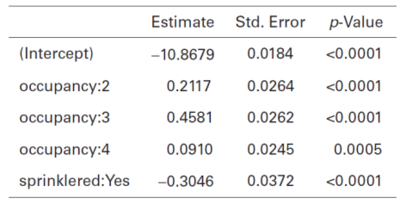
For context, in this problem the GLM is modelling claim frequency using a Poisson distribution with a log-link function and there are two predictor variables, Occupancy Class (1, 2, 3, or 4 with 1 the base level) and Sprinkler Status (with no sprinkler being the base class). It is important to identify the base class for each predictor. Table 1 below is reproduced from the text, it shows the output of a GLM without any interaction term.

Table 1: Model with the main effects of Occupancy Class and Sprinklered Status

To read this table, recall the base class for each variable always has a relativity of 1.000. So only rows for non-base classes are shown. There is a row for each non-base level category in each predictor variable in the model; in general the output looks like "Variable Name: Category". From Table 1 we see any risk in occupancy class 2 (regardless of sprinkler status) has a relativity of [math]e^{0.2117}=1.236[/math] or, phrased differently, a surcharge of 23.6%. For any risk with a sprinkler status of "Yes" the relativity is [math]e^{-0.3046}=0.737[/math] or, phrased differently, a discount of 26.3%.

Under this rating plan, a risk that has a Sprinkler Status of "Yes" and is in Occupancy Class 2 would receive a combined relativity of [math]1.236\cdot 0.737 =0.9109[/math], i.e. a discount of 8.9%.

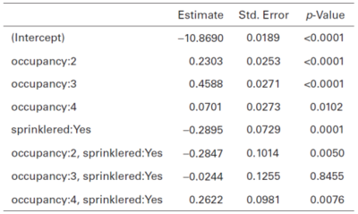
However, we want to go further and test if there is any interaction between the Occupancy Class and Sprinkler Status. For instance, maybe occupancy class 2 involves manufacturing and class 4 involves clerical work. Presumably, having a sprinkler system might help reduce losses in class 2 more than class 4. By telling the GLM software to include the interaction between Occupancy Class and Sprinkler Status, the GLM is building a design matrix with a column for each combination of non-base levels for the variables, so three columns in this case [math]\left((4-1)\cdot(2-1)\right)[/math] [Remember base levels are not counted]. The GLM estimates the coefficient for each of these combinations. Table 2 below is reproduced from the text and shows the GLM output when the interaction is included.

Table 2: The model with the addition of the interaction term

We can tell the model includes an interaction term because Table 2 contains rows which look like "Predictor A , Predictor B", i.e. there is a comma separating the two predictor variables. Without rows like these, the "sprinklered:Yes" row would be referring to all risks which have a sprinkler, regardless of their Occupancy Class.

Since we're including the interaction term, the "sprinklered:Yes" row is referring to risks that have a sprinkler and are in class 1 (the Occupancy Class base). Here, class 1 and sprinklers get a relativity of [math]e^{-0.2895}=0.749[/math], i.e. a 25.1% discount compared to a risk in occupancy class 1 that doesn't have a sprinkler. The p-value of 0.0001 indicates having a sprinkler and being in class 1 is significantly different from being in class 1 and not having a sprinkler.

The key point now is to understand the relativities for the remaining occupancy classes with sprinklers are relative to the occupancy class in question with no sprinklers.

For a risk in occupancy class 2 which has sprinklers, the relativity is [math]e^{-0.2895+-0.2847}=0.563[/math], or a 43.7% discount compared to a risk in occupancy class 2 that doesn't have sprinklers. The p-value of 0.005 indicates there is a significant difference in the indicated magnitude of the sprinkler discount between class 2 and class 1 (43.7% vs 25.1% discount respectively).

Key Point: The order of the predictors is really important. We do not get the same results if we use the occupancy:2 estimated coefficient. In general, for PredictorA and PredictorB, the GLM output looks like PredictorA , PredictorB for an interaction, and this coefficient is relative to the PredictorB variable status because the Predictor A variable is the same in the numerator and denominator of the relativity calculation.

Similarly, for occupancy class 3 with sprinklers, the relativity is [math]e^{-0.2895+-0.0244}=0.731[/math], or a 26.9% discount compared to a risk in occupancy class 3 without sprinklers. However, the p-value is 0.8455 which is greater than the typical 0.05 so this result is not significant. This means we should consider grouping class 3 with sprinklers with risks that are class 1 with sprinklers. However, this doesn't mean we should consider grouping class 3 with class 1 in general because the p-value for Occupancy:3 is <0.0001, i.e. there is a significant difference between the classes when they have no sprinkler.

Lastly, repeating this analysis for occupancy class 4 with sprinklers, we find the relativity is [math]e^{-0.2895+0.2622}=0.973[/math], or a 2.7% discount. While the p-value of 0.0076 does suggest this result is significant, the GLM is saying only a weak discount is merited, so consideration should be given towards not giving a sprinkler discount for risks in occupancy class 4.

Alice: "This material can be a bit confusing and we're still iterating to find the best way to present it. Take a look at the [forum discussion] for more thoughts on this topic."

Interacting a Categorical Variable with a Continuous Variable

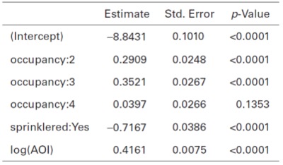
We continue to follow the example in the GLM text by adding a variable called Amount of Insurance (AoI) to the claim frequency model. Since the Amount of Insurance is a continuous variable, it is logged prior to inclusion in the GLM using the natural logarithm, ln(). Further, there is no natural base level for a continuous variable. Table 3 below is from the text and shows the GLM output without the interaction term.

Table 3: A model with Occupancy Class, Sprinklered Status, and Amount of Insurance as main effects

Since there are no interaction terms, this says the presence of a sprinkler gets a relativity of [math]e^{-0.7167}=0.488[/math], and the log of mean claim frequency increases by 0.4161 for each unit increase in the log of the Amount of Insurance. Alternatively, the mean claim frequency is proportional to [math]AoI^{0.4161}[/math].

When we specify the GLM should include an interaction between the sprinkler variable and the log(AoI) variable, the GLM adds a column to the design matrix which is 0 if there is no sprinkler, and is the quantity, log(AoI), if there is a sprinkler. That is, the column is the product of the sprinkler indicator ("Yes"=1) and the log(AoI) columns in the design matrix.

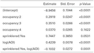
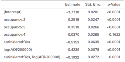
Table 4 below is from the text and shows the GLM output when we include the interaction term.

Table 4: Adding the interaction of AoI and Sprinklered Status

For this model, the log(AoI) curve is in relation to the base class for sprinklers (i.e. No Sprinklers). The coefficient of the interaction term is estimated as -0.1032, so the AoI curve is less steep when sprinklers are present than otherwise. The mean claim frequency curve is proportional to [math]AoI^{0.3207} = AoI^{0.4239+-0.1032}[/math] when there is a sprinkler, and [math]AoI^{0.4239}[/math] when there is no sprinkler.

Care is also needed when interpreting the sprinklered:Yes coefficient. At first glance, the value 0.7447 could imply we should be surcharging for the presence of a sprinkler. This seems counter-intuitive and goes against the results of the model before we included the interaction term. However, we really have two separate Amount of Insurance curves, one for with sprinkler, and one for without. Let's pause our example and investigate a smaller model in more depth.

Let [math]\log(\mu)=\beta_0+\beta_1x_1+\beta_2x_2+\beta_3x_3[/math] be our GLM where x₁ is the Sprinkler variable, x₂ is the [math]\log(AoI)[/math] variable, and x₃ is the interaction of Sprinkler and Amount of Insurance variable.

Writing out the equations for sprinkler or no sprinkler gives:

Risk has no sprinklers	[math]\log(\mu)=\beta_0+\beta_2\log(AoI)[/math].
Risk has sprinklers	[math]\log(\mu)=\beta_0+\beta_1+\beta_2\log(AoI)+\beta_3\log(AoI)= \left(\beta_0+\beta_1\right)+\left(\beta_2+\beta_3\right)\log(AoI)[/math]

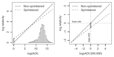
Comparing these equations term by term we see the interaction coefficient, [math]\beta_3[/math], changes the slope of the Amount of Insurance curve for risks with a sprinkler. The coefficient of the main effect, [math]\beta_1[/math], adjusts the y-intercept of the Amount of Insurance curve for risks with a sprinkler. The addition of the interaction term has no impact on the values predicted for risks without sprinklers. These effects are seen in the left hand diagram found of Figure 1 below.

Figure 1: Illustration of the effect of the interaction of Sprinklered and AoI (left panel) and the same model after dividing AoI by its base amount (right panel)

So we understand how the main effect and interaction terms change the Amount of Insurance curve for risks with a sprinkler. However, this doesn't immediately say why the main effect in our example appears to suggest a surcharge.

The key to understanding this is to recall an AoI of $1 is very unlikely in insurance. Normally it would be much higher. It is helpful to re-base the Amount of Insurance curve to a more common value, for instance the median of the distribution. We'll assume the base level in our example is $200,000.

To re-base the Amount of Insurance curve, divide the Amount of Insurance by the Base AoI prior to log-transforming and running the model. When you transform a variable correctly, it won't change the predictions you make but will change the coefficients returned by the GLM.

Let's pause our example again to look at the smaller version. Suppose we re-base to $200,000. Then the GLM looks like [math]\log(\mu)=\gamma_0+\gamma_1y_1+\gamma_2y_2+\gamma_3y_3[/math] where [math]y_1=x_1[/math] is the Sprinkler variable, [math]y_2=\log\left(\frac{AoI}{Base AoI}\right)[/math], and [math]y_3[/math] is the interaction variable.

Again, let's write out the equations for no sprinkler and sprinkler risks.

No sprinkler	[math]\log(\mu)=\gamma_0+\gamma_2\log\left(\frac{AoI}{Base AoI}\right)[/math]
Sprinkler	[math]\log(\mu)=\gamma_0+\gamma_1+\left(\gamma_2+\gamma_3\right)\log\left(\frac{AoI}{Base AoI}\right)[/math]

Comparing with their counterparts above, the no-sprinkler equations show [math]\gamma_2=\beta_2[/math] and [math]\gamma_0=\beta_0+\beta_2\log(Base AoI)[/math]. That is, the slope of the line is the same but the y-intercept has been re-scaled because we re-scaled the Amount of Insurance.

Substituting these into the second sprinkler equation and comparing it then gives [math]\gamma_3=\beta_3[/math] and [math]\gamma_1=\beta_1+\beta_3\log(Base AoI)[/math].

Now using the re-based GLM, but substituting in for the [math]\beta_i[/math] we get

No sprinkler	[math]\log(\mu)=\beta_0+\beta_2\log(Base AoI)+\beta_2\log\left(\frac{AoI}{Base AoI}\right)[/math]
Sprinkler	[math]\log(\mu)=\beta_0+\beta_2\log(Base AoI)+\left(\beta_1+\beta_3\log(Base AoI)\right)+\left(\beta_2+\beta_3\right)\log\left(\frac{AoI}{Base AoI}\right)[/math]

Evaluating these equations at base level sets [math]\log\left(\frac{AoI}{Base AoI}\right)=0[/math]. We can then observe that at the base level, the difference between a risk with sprinklers and a risk without is [math]\beta_1+\beta_3\log(Base AoI)=\gamma_1[/math]. That is, the coefficient of the main effect in the re-based GLM shows the discount received by a risk with sprinklers and base Amount of Insurance.

Returning to the example, this means it's very hard to look at the coefficient of the main effect for an interacted variable and say whether or no they receive a discount. It all depends on where the base is. This is illustrated in the right hand diagram of Figure 1 above. The model coefficients produced by the GLM using the re-based Amount of Insurance variable are shown in Table 5 below.

Table 5: The model of Table 4 with [math]\log(AoI)[/math] centered at $200,000

Question: What are two advantages of re-basing variables to their base level?

Solution:

The intercept term represents the average (frequency/severity/pure premium etc.) at base levels which is intuitive/easier to interpret.
When a variable is not centered on its base level the coefficient of the GLM may have the opposite sign to what is expected. By centering a variable on its base level the GLM coefficients become more intuitive to understand.

Interacting Two Continuous Variables

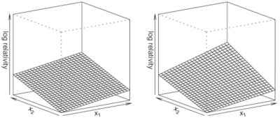
Determining whether or not the interaction term between two continuous variables is significant or not can be done using perspective plots. We produce two perspective plots, one for the model with the interaction term and the other for the model without the interaction term.

A perspective plot graphs the predictors on the x and y axes and the relative log response on the z-axis (see Figure 2 below). The response is relative because each graph is re-scaled to a common scale to allow for easy comparison between them.

If the two predictor plots look significantly different then the interaction term is likely significant. Ultimately, you should use the p-value to help determine significance.