Holmes.PenalizedRegression
Reading: Holmes, T. & Casotto, M, “Penalized Regression and Lasso Credibility,” CAS Monograph #13, November 2024. Chapter 3, Sections 3.1 — 3.3.
Synopsis: We introduce the concept of penalized regression which is an extension of the GLM framework that incorporates a measure of the model complexity. We explore three common types of penalty term (ridge, lasso, and elastic net), looking at how the size of the penalty parameter impacts the beta coefficients for each method. We conclude by arguing why lasso regression is recommended for actuarial purposes and discuss how to choose the optimal penalty parameter.
Study Tips
This is a fairly quick and logical reading which introduces the key ideas underpinning this monograph. Pay close attention to the balance between the number of records in the data set and the number of variables in the model as the optimization process involves juggling both of these at once.
Estimated study time: 4 Hours (not including subsequent review time)
BattleTable
Based on past exams, the main things you need to know (in rough order of importance) are:
- The expressions for the ridge, lasso, and elastic net penalty terms.
- Explain what is meant by a natively sparse statistical model.
- Describe how to perform k-fold cross-validation.
Questions from the Fall 2019 exam are held out for practice purposes. (They are included in the CAS practice exam.)
reference part (a) part (b) part (c) part (d) Currently no prior exam questions
| Full BattleQuiz | Excel Files | Forum |
You must be logged in or this will not work.
In Plain English!
Our goal is to find an actuarially sound way of incorporating credibility into the generalized linear modeling process. We begin by looking at the three most common penalization methods: lasso, ridge, and elastic net. With a GLM we could maximize the log-likelihood for the model or minimize the negative log-likelihood. Penalized regression focuses on minimizing the negative log-likelihood and adjusts the formula to include a penalty term as follows:
[math]\hat{\beta} = {\arg\!\min}_\beta\left[ NLL(y, X, \beta) + \color{red}{\lambda\textrm{Penalty}(\beta)}\color{black}\right]. [/math]
The penalty parameter, [math]\lambda[/math], is a non-negative number. When it is zero, we have a traditional unpenalized GLM. The penalty parameter introduces a trade-off between improving the model's goodness of fit and our prior assumptions about the model structure. In particular, we can choose the penalty to prefer models with desirable properties such as a low number of parameters. As the penalty parameter increases, we give more weight to the a priori structure of the coefficients.
Alice: "I've added [ ] to the above argmin equation to emphasize we must consider both the negative log-likelihood and the penalty term when optimizing the set of beta coefficients. As you work through the concept of penalized regression it's helpful to keep in mind that the NLL is a function of the number of observations in the dataset and the penalty term is a function of the number of parameters in the model. It's a good idea to track the relative size of these because a small improvement on a large number of records (decrease the NLL) may outweigh a significant increase in the penalty term."
Three types of Penalty
- The ridge penalty is the sum of squares (squared [math]l^2[/math]-norm) of [math]\beta[/math]:
[math] \textrm{Ridge}(\beta) = \displaystyle\frac{1}{2}\sum_{j=1}^p \beta_j^2 = \frac{1}{2}\left|\left|\beta\right|\right|_2^2 [/math]
- The lasso penalty is the sum of the absolute values ([math]l^1[/math]-norm) of [math]\beta[/math]:
[math] \textrm{Lasso}(\beta)=\displaystyle\sum_{j=1}^p\left|\beta_j\right| = \left|\left|\beta\right|\right|_1 [/math]
- The elastic net penalty is a linear combination of the ridge and lasso penalties. We choose a parameter, [math]\alpha[/math], such that [math] 0 \lt \alpha \lt 1[/math], then:
[math] \mbox{Elastic Net}_\alpha(\beta) = (1-\alpha)\textrm{Ridge}(\beta) + \alpha\textrm{Lasso}(\beta) = \displaystyle\frac{1-\alpha}{2}\sum_{j=1}^p \beta_j^2 + \alpha\sum_{j=1}^p|\beta_j| [/math]
Alice: "An easy way to remember where the [math]\alpha[/math] parameter goes is lasso contains an a which is the start of alpha. Ridge doesn't contain an a so is the complement."
Penalized regression follows the same approach as modeling using an unpenalized GLM. We still have a link function, linear predictor, and assume the observations follow a predetermined distribution around the estimated parameter. Introducing the penalty term changes the coefficient estimates.
Each of the ridge, lasso, and elastic net penalties are designed to shrink the model coefficients towards zero because they add an increasingly large positive penalty as the coefficients increase in size and we are trying to minimize the sum of the negative log-likelihood and penalty term. The penalty is said to regularize the coefficients.
Important! The penalty is sensitive to the parameterization of the design matrix (feature matrix). For example, the coefficients might be quite large for an annual mileage variable but they might be materially smaller for the same variable when it's expressed in thousands of miles per year.
It's best practice to standardize the features before solving the penalized regression problem. This means rescaling each column of the design matrix, X, to have mean 0 and standard deviation equal to 1.
Most software packages automatically standardize the design matrix for you, solve the penalized regression problem, and then return the unstandardized coefficients. The source text doesn't tell us how to unstandardize the coefficients.
Ridge Regression
Ridge regression is popular become can provide stable estimates in the presence of highly correlated variables. This is an advantage because GLMs become unstable in the sense that the coefficients may become unreasonably large when some variables are highly correlated. The ridge penalty parameter protects against this during the optimization process.
[math]\hat{\beta}_\textrm{Ridge} = {\arg\!\min}_\beta\left[ NLL(y, X, \beta) + \displaystyle\frac{\lambda}{2}\sum_{j=1}^p \beta_j^2\right]. [/math]
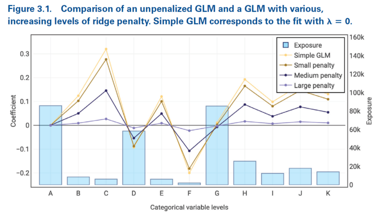
Figure 3.1 below is taken directly from the source material. It demonstrates as the ridge penalty increases, the model coefficients move away from their unpenalized starting point towards closer to zero. Another key insight is for a fixed penalty parameter, the beta coefficients are pulled closer to zero when the underlying exposure is small than when the underlying exposure is large. That is, the amount of shrinkage depends on the underlying exposure volume.
Alice: "Exposure based shrinkage makes sense because when there are few exposures in a category only a few terms contributing to the NLL will change. This means it's easier for the penalty term to increase by more than the NLL decreases, so optimizing the beta coefficients means they should shrink towards zero fast to reduce the size of the penalty term."
In Appendix A.2, Holmes and Casotto demonstrate that under certain conditions there is a direct parallel between ridge regression and Bühlmann credibility whereby Bühlmann's K equals the ridge parameter.
Alice: "In my opinion that part of the appendix is mathematically dense and only applies under certain conditions. It doesn't seem reasonable to test you on it. I'll continue to pull any relevant material out of the appendices for you."
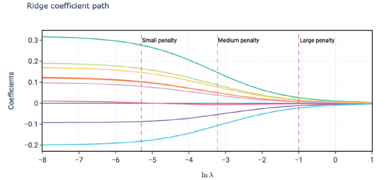
A nice way to observe this is to look at a plot of the coefficient path such as that seen below in Holmes and Casotto's Figure 3.2. Each (standardized) beta coefficient produces a curve called its coefficient path which shows the value of the coefficient as the penalty parameter varies. With ridge regression we see each coefficient begins at its unpenalized value and smoothly and gradually decreases to close to but never quite reaching zero. This nicely parallels Bühlmann credibility where we never quite reach 100% credibility for any given variable.
mini BattleQuiz 1 You must be logged in or this will not work.
Lasso Regression
A fundamentally important feature of lasso regression is achieves sparsity. Sparsity means the process has the ability to set non-significant coefficients equal to zero during the fitting procedure. A nice consequence of this is lasso regression automates both variable selection and the estimation of coefficients.
[math]\hat{\beta}_\textrm{Lasso} = {\arg\!\min}_\beta\left[ NLL(y, X, \beta) + \lambda\displaystyle\sum_{j=1}^p\left|\beta_j\right|\right]. [/math]
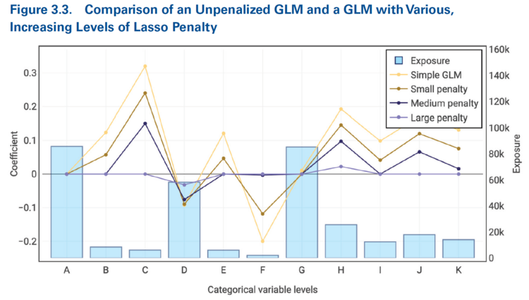
Figure 3.3 from the source text is shown below. Like with ridge regression, the beta coefficients shrink towards zero as the penalty parameter, [math]\lambda[/math] increases. We also see that the shrinkage is greater when the exposure volume is lower. However, the key difference between ridge and lasso regression is the lasso regression sets some coefficients equal to zero. We see this for categories B, C, E, F, and I which each have a zero coefficient once the penalty parameter is medium or large. Notice though that categories J and K have more exposures so their beta coefficients are only forced to zero once we use a "large" penalty parameter.
Alice: "If we are using a log link function then this says the relativity for the category is [math]e^0 = 1.000[/math]."
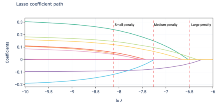
It's even easier to see this when we look at the coefficient path plot for lasso regression (Figure 3.4 below). As with ridge regression, we have smooth, gradual progressions towards zero as the penalty parameter increases. The key difference is for each coefficient there is a value of penalty parameter after which the coefficient is always zero.
One way to view this is for a sufficiently large penalty parameter all of the coefficients will be zero. As we decrease the penalty parameter we pick up non-zero coefficients in the model at different times as they overcome the penalty.
Alice: "There is a significant portion of the appendices devoted to mathematically explaining why lasso regression achieves sparsity through including a non-differentiable penalty term. In my opinion, this material is too technical to be tested on the exam."
Elastic Net Regression
Recall from GLM.Basics that collinearity refers variables which are highly correlated so may be expressed as a linear combination of others. Holmes and Casotto claim that ridge regression will pick up all collinear variables, giving them similar [math]\beta_j[/math] coefficient. In contrast, they claim lasso regression will likely select one of the correlated variables to have a non-zero coefficient.
Elastic Net Regression is a weighted average (convex combination) of the ridge and lasso penalties. We have
[math] \hat{\beta}_{\textrm{Elastic}\,\textrm{net},\, \alpha} = {\arg\!\min}_\beta \left[NLL(y, X, \beta) + \lambda\left(\displaystyle\frac{1-\alpha}{2}\sum_{j=1}^p\beta_j^2+\alpha\sum_{j=1}^p|\beta_j|\right)\right] [/math]
Here, [math]\lambda[/math] is still our chosen penalty parameter. However, we have introduced a hyperparameter, [math]\alpha[/math]. Holmes and Casotto do not define what they mean by a hyperparameter but in machine learning it's commonly used to refer to a parameter whose value is set before the modeling/learning process begins rather than being learned/determined during training. According to Holmes and Casotto, [math]\alpha[/math] depends on the nature of the data and the process of computing it is beyond the scope of the monograph.
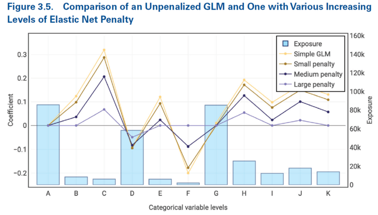
Figure 3.5 below is taken directly from the source material and shows how elastic net regression has the following attributes:
- The beta coefficients approach zero as the penalty parameter increases.
- When the penalty parameter is sufficiently large, it is possible for a coefficient to be exactly equal to zero.
- Categories with lower exposure volumes have their coefficients approach zero more quickly as the penalty parameter increases than those which have a greater volume of exposures.
It's particularly helpful to directly compare Figures 3.3 (lasso regression) and 3.5 (elastic net regression). When using lasso regression we saw the coefficients for categories B, C, E, F, and I were zero for medium and large penalty parameters. When using elastic net regression with the same penalty parameters, we now see categories C, F, and I have non-zero coefficients for the medium penalty parameter and C's coefficient remains non-zero even when the penalty parameter is large. This is because of the choice of the hyperparameter, [math]\alpha[/math], which pushes out the point at which the coefficient goes to zero.
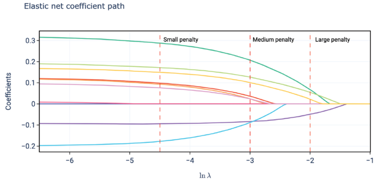
It's illustrative to do the same with the plot of the coefficient paths which, for elastic net regression, is shown below in Figure 3.6. At first glance, this plot looks identical to the corresponding lasso plot (Figure 3.4). Closer inspection shows the key difference is the position of the x-axis. The points at which the coefficients become zero under elastic net regression occurs significantly further along the x-axis than they did under lasso regression. Further, contrasting with Figure 3.2 (ridge regression), we see the elastic net has resulted in all of the coefficients shown going to zero at a point on the x-axis which is prior to where they had materially converged to zero under ridge regression.
Why Lasso Regression is Recommended for Actuarial Applications
A sparse statistical model is one which has only a small number of non-zero coefficients. It follows the idea of parsimony — less is more — because the simplicity of a sparse model likely makes it easier to interpret/explain to others.
A statistical model which has the ability to automatically set coefficients equal to zero is known as a natively sparse model. Thus, lasso regression is a natively sparse model while ridge regression is not.
Question: Briefly describe three desireable outcomes of using a sparse statistical model for actuarial purposes.
- Solution: Sparse actuarial pricing models are:
- More stable over time — avoiding constant changes in pricing characteristics is valued by policyholders, regulators, and insurers (reducing filing and IT expense for example).
- Easier to interpret — internal stakeholders and regulators can more readily assess if the proposed model logically achieves the desired outcomes. Policyholders may find it easier to understand why their premium changed overtime.
- Less reliant on judgment because they automatically set a statistical materiality standard. This is because variables only appear in the model once they become material/significant. This greatly helps set the boundary between modeling and model review.
Question: Briefly describe why lasso penalization is preferred over ridge or elastic net penalization for actuarial purposes.
- Solution: Lasso penalization is more responsive to significant coefficients than either ridge or elastic net penalization. This is because ridge penalization has coefficient curves which are convex (grow slowly) when the coefficient initially becomes significant (see Figure 3.2). Whereas lasso penalization produces coefficient curves that are concave (grow rapidly, see Figure 3.4) once the coefficient becomes significant/passes the threshold of materiality. While elastic net penalization also exhibits concave behavior, the elastic net coefficients grow slower than the lasso coefficients (contrast the x-axis scale for Figure 3.4 and Figure 3.6 to see this).
Selecting the Penalty Parameter
The penalty parameter, [math]\lambda[/math], plays a critical role in the model. Actuarial judgment is critical and may be used to place greater weight on the complement of credibility or a prior assumption through selecting a larger penalty parameter than statistically indicated.
There is no analytic/explicit formula to calculate the correct value for the penalty parameter. In general, the model is fitted for a range/selection of penalty parameters and then the best model is chosen.
Question: How do we define "the best model"?
- Solution: The best model is one which generalizes well to unseen data. We can apply a statistical quality of fit such as the Gini coefficient or deviance measure to the model output when it is given an unseen dataset. The best model is the one which produces the best statistical quality of fit - i.e. has the best generalized predictive power.
k-Fold Cross-Validation
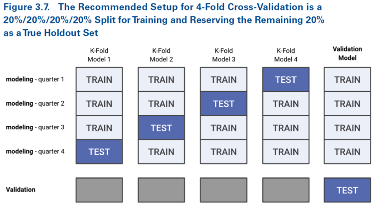
k-fold cross-validation is a way of simulating model behavior on an unseen data set. The initial dataset is partitioned into two sets; the modeling set (aka training set) and the validation set. The modeling set is itself divided into k equal parts with k = 4 being common.
For k-fold cross validation there are k ways to choose one part from the set of parts which make up the modeling set. For each of these k ways we train our model on the remaining k - 1 data sets (folds) and use the kth fold (the test fold) to measure its performance via metrics such as deviance, Gini coefficient, and pseudo-R2. Holmes and Casotto say these metrics can then be combined to estimate the performance of the penalty parameter on unseen data but they do not go into the details of how to do so.
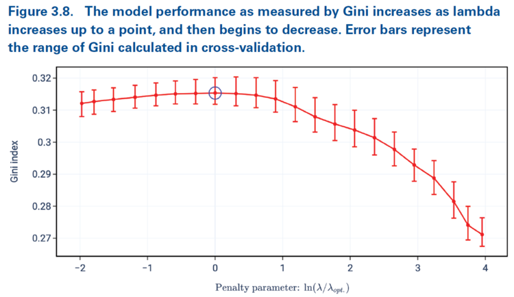
Alice: "My understanding is you can run k-fold cross-validation a number of times using various penalty parameters. You can then plot say the range of Gini coefficients for a given penalty parameter and look for the penalty parameter which maximizes your metric. Holmes and Casotto demonstrate this in Figure 3.8 below."
The red bars in Figure 3.8 show the range of outcomes of the k-fold cross-validation metric for a given penalty parameter. The red dots indicate the mean outcome. Our goal is to choose the penalty parameter which maximizes our chosen performance measure (Gini coefficient in this case). It's possible, as seen here, that while there may be an optimal penalty parameter, other values may exhibit similar performance.
In Figure 3.8 above, the x-axis has been rescaled using a function of the optimal penalty parameter. In practice you would do this after selecting your penalty parameter (the optimal one). The rescaling allows you to confirm you've picked the best one. Cross-validation provides a range of viable penalties and it's up to the modeler/actuary to pick the best one, taking into consideration the overall reasonability of the model output and other actuarial considerations. Actuarial judgment is sometimes used to select a slightly higher than optimal penalty parameter to place more weight on the complement of credibility.
After selecting our penalty value we combine all k-folds together and train our model again using the full modeling data set. Finally we can then measure the overall model performance using the as yet unseen validation set. Holmes and Casotto's Figure 3.7 below shows this in action.
It's critically important to measure model performance on a data set that has not been seen by either model (say current and proposed).
| Full BattleQuiz | Excel Files | Forum |
You must be logged in or this will not work.
