Fisher.Visualization

Reading: Fisher, G. et al, "Individual Risk Study Note," CAS Study Note, Version 3, October 2019. Chapter 3. Section 2

Synopsis: In this section we look at how to illustrate characteristics of policies with either an aggregate limit, per-occurrence limit or both. We derive a key formula for the base premium used in retrospective rating and a pair of equations which relate the maximum and minimum premiums to the entry ratios.

Forum

Study Tips

This is a fairly challenging topic to understand, not least because it requires you to get used to thinking about data in a different way to usual. You can right click on any of the figures to open them in a new browser tab at full size.

Since this topic comes up frequently it's worth returning to this article several times and repeatedly tackling the exam questions.

Estimated study time: 1 week (not including subsequent review time)

BattleTable

Based on past exams, the main things you need to know (in rough order of importance) are:

• Lee Diagrams - understand the concept and be able to draw them.
• Balance Equations - know the formulas and be able to apply them.
• Lee Diagrams - layer & size methods for calculating insurance charges and savings.
• Lee Diagrams & Retrospective Rating - know the key formula and be able to apply it.

Questions are held out from Fall 2019 exam. (Use these to have a fresh exam to practice on later. For links to these questions see Exam Summaries.)

reference	part (a)	part (b)	part (c)	part (d)
E (2017.Fall #12)	Lee Diagrams - draw	Lee Diagrams - layer & size methods	Size & Layer Methods - Fisher.TableM	Lee Diagrams - concepts
E (2016.Fall #13)	Lee Diagrams - insurance charge	Balance Equations - calculate
E (2016.Fall #14)	Lee Diagrams - concepts	Tables L & M - Fisher.TableL	Tables L & M - Fisher.TableL
E (2015.Fall #7)	Lee Diagrams - layer method	Lee Diagrams - size method	Lee Diagrams - ILFs	Consistency Test - Bahnemann.Chapter6
E (2015.Fall #14)	LDD Premium - Fisher.CaseStudy	Lee Diagrams - concepts
E (2015.Fall #17)	Balance Equations - calculate	Retrospective Premium - Fisher.ExpRating
E (2014.Fall #16)	LDD Plan - Fisher.CaseStudy	Lee Diagrams - concepts	Table M - Fisher.TableM
E (2014.Fall #18)	Balance Equations - calculate
E (2013.Fall #7)	Lee Diagrams - excess ratio	Lee Diagrams - dispersion (outdated)	Lee Diagrams - dispersion (outdated)
E (2013.Fall #14)	Lee Diagrams - retrospective rating
E (2013.Fall #15)	Lee Diagrams - concepts	Lee Diagrams - concepts	Lee Diagrams - concepts
E (2012.Fall #19)	Lee Diagrams - retrospective rating	Retrospective development - Fisher.ExpRating
E (2012.Fall #21)	Lee Diagrams - insurance savings	Lee Diagrams - concepts

Full BattleQuiz You must be logged in or this will not work.

Forum

In Plain English!

When working with per-occurrence limits and aggregate limits it can be helpful to visualize them. A widely used approach to visualizing them was developed in a paper by Yoong-Sin Lee .

Alice: "Lee's paper isn't on the syllabus itself, but sometimes with tricky material it helps to refer to the original source."

The graphs described in the paper are usually referred to as "Lee diagrams". A Lee Diagram has the cumulative claims (count or percentage of loss distribution) on the horizontal axis, and the severity, aggregate loss or entry ratio (the "size") on the vertical axis. Let's look at this in more detail.

Let n be the number of losses, let the loss sizes be x₁, ..., x_q and assume they're ordered such that x₁ < x₂ < ... < x_q. Let the associated loss frequencies be given by n₁, ..., n_q thus n = n₁ + ... + n_q.

Figure 1 below shows the more traditional way of viewing a sample of 10 claims. Notice how in the second part of the figure we've ordered the claims by loss size and added the incremental and cumulative counts. So here x₁ = 1, x₂ = 2, ..., x₁₅ = 15 and n₁ = 2, n₂ = 0, ..., n₁₅ = 2, and n = n₁ + ... + n₁₅ = 10.

Figure 1

When we produce a diagram like Figure 1 we are asking ourselves: "For a fixed size of loss, how many claims (count or percentage) are smaller than this loss size?"

To draw a Lee diagram we need to turn this question around and ask: "What is the size of loss that k% of claims are smaller than?"

Figure 2 below shows a Lee diagram of the ten claims used in Figure 1 above. To sketch this, order the losses (the x_i's) from smallest to largest. Let k be either the cumulative claim count or the percentage of claims, in the latter case the horizontal axis will be scaled between 0 and 1. For each value of k find the value q such that [math]\displaystyle\sum_{i=1}^{q-1} n_i \leq k \lt \displaystyle\sum_{i=1}^q n_i[/math]. Plot the point (k, x_q).

For example, there are 10 claims in Figure 1. Letting k = 5 we see that the cumulative claim count column goes directly from 2 to 6, which means q = 3. This means we plot the point (5, x₃) = (5, 3) on the Lee diagram. Since we're dealing with discrete data we get a step function, with the next value being (6, 5) as the next claim size is 5 and when we reach that we've incurred six claims.

Figure 2

Notice in Figure 2 above that the green shaded area is a rectangle of height 3 and width 4. This corresponds to the incremental number of claims for claim size three. So an easier way of remembering to draw a Lee diagram is to order the claims by size and then draw successive rectangles whose height is the claim size and width is the number of claims of that size. Lastly, observe the area of the green shaded rectangle is the same as the total cost of all claims of size 3.

Figure 3 below generalizes this idea to the continuous case where a small change in cumulative probability, dF(x), corresponds to losses of size between x and x + δx. Then the vertical strip represents xdF(x) which is the expected loss of the strip. Summing these infinitely small strips gives the expected value [math]E[X]=\displaystyle\int_0^\infty x\mathrm{d}F(x)[/math]. Observe F(x) goes from 0 to 1 but dF(x) goes from 0 to [math]\infty[/math] because to change F(x) we must move the underlying loss between 0 and positive infinity.

Figure 3

Summing over the cumulative claim count/integrating over all claims yields the total expected loss dollars incurred by the insurer. Switching to summing/integrating over the cumulative claim count distribution yields the expected loss per policy incurred by the insurer. Normalizing the horizontal axis to a percentage gives a per loss basis.

Applying a per-occurrence limit L

Figure 4 below is a Lee diagram when there is a per-occurrence limit L on the policy. The shaded area represents the expected payment per loss because the horizontal axis is the cumulative claim count percentage.

Losses of size x₁ < L are paid out in full whereas losses x₂ > L are paid out at L.

Figure 4

Applying a per-occurrence deductible D and limit L

Figure 5 below shows a Lee diagram when there is both a per-occurrence deductible D and a per-occurrence limit L on the policy. The payout per claim is best expressed as follows

[math]\mbox{payout} = \begin{cases} 0 \mbox{ (No payout)} & x \lt D\\ x-D &D \lt x \lt L \\ L-D &L \lt x \end{cases} [/math]

The shaded area is the expected payout per loss under both the deductible and limit.

Figure 5

Calculating with Lee Diagrams

You can calculate the area of the shaded region in a Lee diagram using integration along either of the axes. Alice: "Remember, just like in Calc III, one way may be easier than the other."

First, consider the size method which is where we integrate along the horizontal axis by adding up lots of infinitely small vertical strips to form the shaded area (see Figure 6 below). Each strip has width δF(x) and height x. This gives [math]E[X]=\displaystyle\int_0^\infty x\mathrm{d}F(x)[/math]. Again, remember for F(x) to go between 0 and 1, the size of loss, x, must range between 0 and positive infinity.

Figure 6

Figure 7 below explains why this is known as the size method. Given F(x₁) and F(x₂) we're only considering the expected value of claims between x₁ and x₂ in size, that is, not all claims are considered.

Figure 7

Now consider the layer method which is where we integrate along the vertical axis by summing up infinitely small horizontal bands to form the shaded area (see Figure 8 below). Each band has height δx and width [math]1-F(x)=S(x)[/math] where S(x) is the survival function for F(x). This yields the expected loss per claim (the shaded area) as [math]E[X]=\displaystyle\int_0^\infty 1-F(x)\mathrm{d}x = \int_0^\infty S(x)\mathrm{d}x[/math].

Figure 8

Figure 9 below shows why this is called the layer method because given a layer of claims [x₁, x₂] it considers all claims but only computes the expected loss contributed between x₁ and x₂, i.e. only considers the part of the loss within the layer.

Figure 9

Returning to the idea of a policy with a per-occurrence deductible D and per-occurrence limit L we observe the layer method gives [math]E[X]=\displaystyle\int_D^L S(x)\mathrm{d}x[/math] relatively easily (see Figure 10). Yet to calculate this using the size method we have to compute and add together the green and yellow shaded areas in Figure 10. This area may be expressed using the survival function as [math]E[X]=\displaystyle\int_{F(D)}^{F(L)}x\mathrm{d}F(x) - D\left[S(D)-S(L)\right]+\left(L-D\right)S(L) = \displaystyle\int_{F(D)}^{F(L)}x\mathrm{d}F(x) -DS(D)+LS(L)[/math]. You arrive at the same result if you think in terms of F rather than S but the algebra is a little more involved.

Figure 10

Aggregate Policy Provisions

So far we've visualized the severity distribution of a single claim subject to a per-occurrence limit and a deductible. Now we'll consider the impact of applying aggregate policy provisions. Our goal now is to understand and estimate aggregate excess losses. We'll do this first by assuming there is an aggregate limit and no per-occurrence limit.

We may think of the aggregate loss distribution as the result of many simulations of a loss on a single policy. Previously, we calculated and visualized the expected loss for a single claim. Thus, since we know the result of the simulation (the actual loss), we can form an entry ratio [math]r=\frac{\mbox{actual loss}}{\mbox{expected loss}}[/math] for each simulation (see Fisher.AggExcess). We then proceed as before by ordering the entry ratios from smallest to largest and plotting the distribution. The horizontal axis remains the cumulative claim count (cumulative entry ratio) percentage, while the entry ratio is plotted on the vertical axis (see Figure 11).

For a given entry ratio, r, we can draw the insurance change and insurance savings on the Lee diagram (see Figure 12). Recall from Fisher.AggExcess, the insurance charge is [math]\phi(r)=\displaystyle\int_r^\infty \left(y-r\right)f(y)\mathrm{d}y[/math] and this corresponds to the green shaded region. Similarly, the yellow shaded region is [math]\psi(r)=\displaystyle\int_0^r\left(r-y\right)\mathrm{d}F(y)[/math], where F is the cumulative aggregate loss distribution.

• 

  Figure 11

• 

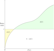
  Figure 12

• 

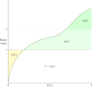
  Figure 13

Key Points

1. The area under the cumulative aggregate loss distribution is 1.
2. φ(r) decreases as r increases, i.e. [math]\phi(r)\rightarrow 0 \mbox{ as } r\rightarrow \infty[/math]
3. ψ(r) is an increasing function of r, i.e. [math]\psi(r) \rightarrow 0 \mbox{ as } r\rightarrow 0 \mbox{ and } \psi(r)\rightarrow\infty \mbox{ as } r\rightarrow\infty[/math].
4. [math]\phi^\prime(r) = -S(r), \phi^{\prime\prime}(r)=f(r)[/math]
5. [math]\psi^\prime(r) = F(r), \psi^{\prime\prime}(r)=f(r)[/math]
6. Key Formula: [math]\color{red}\psi(r)=\phi(r)+r-1[/math].

These points are illustrated in Figures 12 and 13 above. Points 4 and 5 are derived by analyzing small horizontal strips.

Minimum and Maximum Ratable Loss

In experience rating it's common to find a minimum and/or maximum ratable loss; these are used to stabilize premiums from being extremely low or high. We can express the minimum and maximum ratable losses in terms of the entry ratio multiplied by the expected loss E; the minimum ratable loss is rE and the maximum ratable loss is sE for some r < s. Then letting A be the actual aggregate loss gives the aggregate ratable loss as [math]L = \begin{cases} sE & \mbox{if }A \gt sE\\ A & \mbox{if }rE \lt A \lt sE\\ rE & \mbox{if } A \lt rE. \end{cases} [/math]

Figure 14

On our Lee diagram this looks like the green and yellow shaded area in Figure 14 which is the ratio of the expected aggregate loss to expected loss. The actual aggregate losses with entry ratios above s are capped at sE while actual aggregate losses with entry ratios below r are brought up to rE. Thus, [math]\left[1-\phi(s)\right]\cdot E[/math] represents applying the maximum ratable loss and [math]\psi(r)\cdot E[/math] is the additional cost from the minimum ratable loss. This yields the following important formula [math]\color{red}\mathbf{\frac{E[L]}{E}=1+\psi(r)-\phi(s)}[/math]. Here E[L] is the expected aggregate ratable loss and E is the expected loss.

Since a minimum and/or maximum ratable loss can be applied to a policy independent of whether the policy has a per-occurrence limit/deductible, an aggregate limit/deductible, or both, it's important to remember to relate the expected loss, E, and the entry ratios to the type of policy you're pricing. The Fisher text isn't very good at doing this because it's trying to convey the idea in full generality. You should remember if you're pricing a per-occurrence policy using a limited Table M approach then E is really E[A_D], plus the insurance charge and savings are really [math]\phi_D(s)[/math] and [math]\psi_D(r)[/math]. Otherwise, if you're using a Table M approach (aggregate limit/deductible only) or Table L approach (both types of limit/deductible) then E = E[A] and the insurance charge and savings follow their respective definitions.

The Balance Equations

WARNING: What follows diverges slightly from the Fisher text — Alice found the Fisher text tries to do too much all at once so broke it out into three cases and explicitly handles the tax multiplier for you.

Alice: "We've been following the order of material in Fisher. However, this section may make more sense if you skim this section then read the sections on Table M, Limited Table M, and Table L before returning here to battle with the details."

The basic premium is defined as B = bP where P is the standard premium (see Fisher.ExpRating) and b is the basic premium ratio.

In Fisher.RiskSharing we learned the retrospective premium, R, is given by [math]R=\left(B+cL\right)\cdot T[/math] where T is the tax multiplier, c is the loss conversion factor, L is the ratable loss, and B is the base premium. By taking the expectation of each side we get [math]E[R]=(B+cE[L])T[/math] as we assume taxes are always known and E[L] is the expected ratable loss. Our goal is to derive a convenient formula for B.

According to Fisher, when retrospective rating was first introduced it was desirable for a retrospective rating plan to cover its expected losses, expenses and taxes irrespective of the choice of retrospective rating parameters. In full generality this means [math]E[R] = (e+E)\cdot T[/math], where e represents the expenses, and E is the expected loss associated with the plan. Such a retrospective rating plan is known as a balanced plan.

Table M Balance Equations

In the case where the retrospective rating plan only has an aggregate limit/deductible along with the minimum and maximum ratable losses we can use the Lee diagram in Figure 14 above to get:
[math]\begin{align}E[L]&=E[A]+E[A]\cdot\psi(r)-E[A]\cdot\phi(s)\\ &= E[A]-E[A]\cdot\left(\phi(s)-\psi(r)\right) \\&= E[A]-I\end{align}[/math]

where r is the entry ratio for the minimum ratable loss and s is the entry ratio for the maximum ratable loss. I is known as the net insurance charge.

Alice: "Notice there's room for confusion here - as defined above the net insurance charge is in dollars because E[A] is embedded within I. You might be asked for the net insurance charge directly from the Table M (or given it) in which case it's just [math]\phi(s)-\psi(r)[/math]."

In a balanced plan we can equate the two expressions for E[R] above to get [math](B+cE[L])\cdot T=(e+E[A])T[/math]. Then substituting in E[A] - I for E[L] and rearranging yields the following key equation for the Table M basic premium: [math]\color{red}B=e-(c-1)E[A]+cI[/math].

We can go further and derive two key formulas which relate the entry ratios to the defining plan parameters which are the minimum premium H and the maximum premium G.

1. [math]\color{red}\phi(r_H)-\phi(r_G)=\displaystyle\frac{(e+E[A])T-H}{cE[A]T}[/math]
2. [math]\color{red}r_G-r_H = \displaystyle\frac{G-H}{cE[A]T}[/math]

These formulas are known as the Table M balance equations.

Derivation of the Table M balance equations

Limited Table M Balance Equations

The the situation where there is a per-occurrence limit/deductible is more complicated. Recall from Fisher.LimitedTableM that the Limited Table M approach is used to separately price the cost of the per-occurrence limit from the aggregate limit. Further, remember the loss conversion factor, c, is meant to load the losses for loss adjustment expenses (i.e. expenses which vary with the loss volume). We can split these expenses into those associated with the per-occurrence limit loss cost and those associated with the aggregate limit loss cost. Assuming we include the associated load for the per-occurrence limit loss adjustment expenses in the pricing of the per-occurrence limit then we only need load for expenses associated with the aggregate limit when pricing the aggregate limit.

This means when pricing the aggregate limit separately the equation for a balanced retrospective plan with a per-occurrence limit and aggregate limit where each piece is priced separately is [math]E[R]=(e+E[A_D])\cdot T[/math]. We can modify the approach taken in Figure 14 above to write the expected ratable loss as [math]E[L] = E[A_D]\cdot\left(1 - [\phi_D(s) - \psi_D(r)]\right)[/math]. With one important caveat (see below) this yields the Limited Table M basic premium equation: [math]B= e-(c-1)E[A_D]+cI_D[/math].

In this equation it's important to observe that while I_D is still called the net insurance charge it is calculated slightly differently. In this situation we have [math]I_D=E[A_D]\cdot(\phi_D(s)-\psi_D(r))[/math].

CAVEAT : The above formula for the Limited Table M basic premium does not include any provision for losses and associated LAE in excess of the per-occurrence limit/deductible. According to Fisher (p.19), basic premium may or may not include a charge for losses in excess of the per-occurrence limit/deductible. To include a charge for the losses excess of the per-occurrence limit/deductible recall from Fisher.LimitedTableM that we price the per-occurrence limit using [math]E[A]-E[A_D][/math]. Then defining the excess ratio as [math]k=\frac{E[A]-E[A_D]}{E[A]}=1-\frac{E[A_D]}{E[A]}[/math] gives the converted per-occurrence charge as [math]c\cdot k\cdot E[A][/math], where you must remember to convert the charge to account for the plan paying expenses on all claims, not just the part below the limit/deductible which was used to price the aggregate limit. Since we're now including the (expense loaded) price of the per-occurrence limit in basic premium - i.e. within the retrospective rating formula - we're back to the original balanced retrospective plan formula. Namely, [math] E[R] = (B+cE[L])\cdot T = (e +E[A])\cdot T[/math]. Here, it's important to note the use of E[A] as we're accounting for all losses rather than solely those used to price the aggregate limit. Rearranging to solve for the basic premium, B and substituting in [math]E[L] = E[A_D]\cdot (1 - [\phi_D(r_G) - \psi(r_H)])[/math] where rG and rH are the entry ratios associated with the aggregate limit gives: [math]\begin{align}B&=e + E[A] - c\cdot E[A_D]\left(1-[\phi_D(r_G)-\psi(r_H)]\right) \\ &= e - (c-1)E[A] + cE[A] - cE[A_D] + cI_D) \\&= e - (c-1)E[A] + cI_D + c\left(\frac{E[A]-E[A_D]}{E[A]}\right)E[A] \\ &= e - (c-1)E[A] + c(I_D + kE[A]) \end{align}[/math] Hence when including the per-occurrence charge within the basic premium formula we have: [math]B= e-(c-1)E[A]+c(I_D+k\cdot E[A])[/math].

Continuing in the same vein as before, the Limited Table M balance equations are:

1. [math]\color{red}\phi_D(r_H)-\phi_D(r_G)=\displaystyle\frac{(e+E[A])T-H}{cE[A_D]T}[/math]
2. [math]\color{red}r_G-r_H = \displaystyle\frac{G-H}{cE[A_D]T}[/math]

Derivation of the Limited Table M balance equations

Table L Balance Equations

Lastly, in the case where there's both a per-occurrence limit/deductible and an aggregate limit/deductible you follow the same process as before but use the Table L insurance charge, [math]\phi_D^\star(s)[/math], and Table L insurance savings, [math]\psi_D^\star(r)[/math] instead. You're also back to using E[A] instead of E[A_D].

Again, the basic premium may or may not include a charge for losses in excess of the per-occurrence limit/deductible and/or aggregate limit/deductible. The Table L basic premium equation is [math]B= e-(c-1)E[A]+cI_D^\star[/math], where [math]I_D^\star[/math] is again called the net insurance charge but is calculated as [math]I_D^\star=E[A]\cdot(\phi_D^\star(s)-\psi_D^\star(r))[/math]. Since we're pricing the per-occurrence and aggregate limit/deductible simultaneously when using a Table L, we don't have to worry about whether to include an additional term for losses excess of the per-occurrence piece.

The Table L balance equations are:

1. [math]\color{red}\phi_D^\star(r_H)-\phi_D^\star(r_G)=\displaystyle\frac{(e+E[A])T-H}{cE[A]T}[/math]
2. [math]\color{red}r_G-r_H = \displaystyle\frac{G-H}{cE[A]T}[/math]

Derivation of the Table L balance equations

Summary

You should notice the similarities and the differences between the three types of balance equations and the basic premium equations. You should recall the type of expected loss embedded within the dollar version of each net insurance charge. You should be able to identify whether or not to include a charge for losses in excess of a per-occurrence limit/deductible. You should know [math]e - (c-1)E[/math], where E is either E[A] or E[AD] as appropriate, is the called the expense portion of the basic premium. You should know in each set of balance equations the first equation is only true if the plan is balanced. The second equation is true irrespective of whether or not the plan is balanced. Although the entry ratios at maximum and minimum premium have the same notation in each set of balance equations, you need to remember to calculate them using the correct entry ratio definition for the method you're using. See Fisher.AggExcess for a refresher if needed.

Alice: "Still with me? Here are a few tips for memorizing the balance equations:"

1. In the first balance equation the only thing that changes on the right hand side is the expected loss used in the denominator. On the left hand side only the definition of how the entry ratio is calculated changes along with the table used to look up the associated values.
2. In the second balance equation the left and right side have the same pattern of G - H.
3. If you remember the second balance equation then you can remember to flip the order of r_G and r_H when used in the left side of the first balance equation.

Full BattleQuiz You must be logged in or this will not work.

Forum